Stock Overnight Trading Ranking
05 May 2021Contact me for possible collaborations on this project.
This post talks about a stock trading strategy developed by me — ranking stocks based on statistical data of recent stock prices, over the full range of all available stocks on NASDAQ and NYSE. With this strategy you buy stocks in the afternoon, then sell them on the next day’s morning, so I call it overnight trading to distinguish from day trading.
From observing the stock data, I know stock prices fluctuate most between 14:30 and 10:30 the next day. So I wanted to explore the strategy of buying shares at 14:30, and then selling the next day at 10:30. The goal is to maximize stock trading profit by choosing the stocks that will have the best gains from 14:30 to 10:30.
The screenshot below shows what the end result of the project looks like:
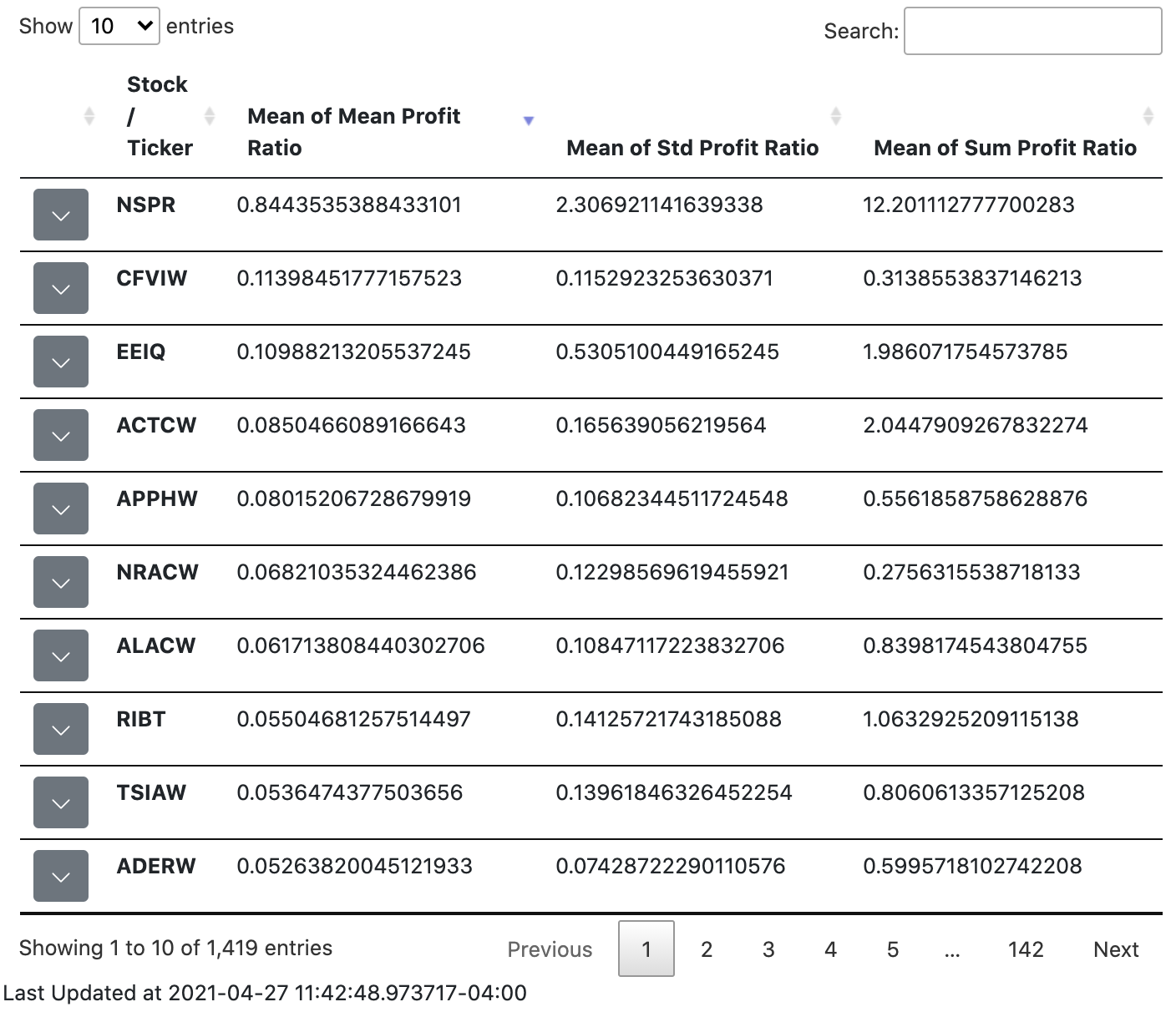
To see how I got there, we’ll first take a look at where to get the data from.
Acquiring Data
Before getting the stock prices for all of the tickers, I need to download all of the stock (ticker) names. I fetch all of the ticker names from nasdaqtrader.com via FTP, and read it in via Pandas. See the code below:
def get_all_tickers():
    subprocess.call('curl ftp://ftp.nasdaqtrader.com/SymbolDirectory/nasdaqlisted.txt > nasdaq_stocknames1', shell = True)
    subprocess.call('curl ftp://ftp.nasdaqtrader.com/SymbolDirectory/otherlisted.txt > nasdaq_stocknames2', shell = True)
    stocknames1 = pd.read_csv('nasdaq_stocknames1', delimiter = '|')
    stocknames2 = pd.read_csv('nasdaq_stocknames2', delimiter = '|')
    stocknames1 = stocknames1.loc[stocknames1['Test Issue']=='N',:] # get rid of Test Issue = Y
    stocknames2 = stocknames2.loc[stocknames2['Test Issue']=='N',:]
    stocknames1 = stocknames1['Symbol']
    stocknames2 = stocknames2['ACT Symbol']
    # sort alphabetically
    # set finds unique items in the list, and combine them together
    return sorted(list(set(list(stocknames1) + list(stocknames2))))
Then, it is time to download the recent stock prices for all of the tickers. To download the stock prices, I used the API provided by Yahoo finance which can be accessed by the yfinance package. See the code below:
def download_from_yahoo(tickers, start, end, interval):
    # tickers is a list of the tickers we want to download stock prices for
    # start and end are datetime objects specifying the time range to download
    # interval is typically '60m', indicating we want data every hour
    print('downloading {} stocks from {} to {}'.format(len(tickers), start, end))
    return yf.download(tickers, start=start, end=end, interval=interval)
The downloaded raw data containing all of the time points looks like this:
Raw data:
                               A       ...    ZYXI
Datetime                               ...
2019-04-29 09:30:00-04:00   77.470001  ...  5.500000
2019-04-29 10:30:00-04:00   77.900002  ...  5.500000
2019-04-29 11:30:00-04:00   78.239998  ...  5.489900
2019-04-29 12:30:00-04:00   78.050003  ...  5.460000
2019-04-29 13:30:00-04:00   77.930000  ...  5.480000
...                            ...     ...    ...
2021-04-27 11:30:00-04:00  137.119995  ...  16.209999
2021-04-27 12:30:00-04:00  137.059998  ...  16.059999
2021-04-27 13:30:00-04:00  137.119995  ...  16.200001
2021-04-27 14:30:00-04:00  136.940002  ...  16.254999
2021-04-27 15:30:00-04:00  136.889999  ...  16.250000
Preprocessing Data
Since I want to see the recent overnight gains between 14:30 and 10:30 the next day (since that is the trading strategy), I selected stock prices at 14:30 and at 10:30 the next day, and organized the data into a Pandas dataframe indexed by date. See below:
Transformed data:
           10:30                 ...     14:30
             AAA     AACQ AACQU  ...     ZWRKW         ZY     ZYNE
Datetime                         ...
2019-04-29   NaN      NaN   NaN  ...       NaN        NaN  11.5400
2019-04-30   NaN      NaN   NaN  ...       NaN        NaN  12.0300
2019-05-01   NaN      NaN   NaN  ...       NaN        NaN  11.8900
2019-05-02   NaN      NaN   NaN  ...       NaN        NaN  10.9550
2019-05-03   NaN      NaN   NaN  ...       NaN        NaN  11.3900
...          ...      ...   ...  ...       ...        ...      ...
2021-04-21   NaN   9.9750   NaN  ...       NaN        NaN   3.9900
2021-04-22   NaN   9.9686   NaN  ...  0.734999  36.180000   4.1050
2021-04-23   NaN  10.0100   NaN  ...       NaN  39.220001   4.1992
2021-04-26   NaN  10.0400   NaN  ...  0.800000  43.369999   4.4712
2021-04-27   NaN  10.2090   NaN  ...  0.750000  45.115002   4.4200
Once the data is in this format, I can use Pandas to quickly compute means, standard deviations, etc. of overnight profit ratios over various time periods (1 week, 1 month, etc.).
Results and Website
The data downloading, preprocessing, and statistical computations are set to run everyday by the server. As shown in the first screenshot (the table is made by using jQuery and the fantastic DataTables library), I used Flask to make a website to display the statistical metrics including mean profit ratio, standard deviation profit ratio and sum profit ratio of daily price differences at 14:30 and 10:30. The table lets you sort by each metric, and you can also search by ticker.
Side Note: Predict stock price overnight differences using Machine Learning Models
I was also curious to see if I could use any machine learning models to predict the overnight price differences. To prepare the data for all of the models I will try, I converted the data into a dataframe containing 6 overnight price differences in a row:
[[-0.0188893 -0.0118471 -0.0007845 -0.0214146 -0.0200625 -0.023225 ]
 [-0.0269201 -0.0147572  0.0047904 -0.0237999 -0.0144927 -0.018867 ]
 [-0.0165142 -0.0078225  0.0105189 -0.011818  -0.0096197 -0.026127 ]
 ...
 [ 0.0100107  0.0067447  0.0133380  0.018402   0.0309677 -0.009351 ]
 [ 0.0377588  0.038293   0.0251833  0.0228506 -0.0392106 -0.027952 ]
 [ 0.0219882  -0.007765 -0.0157289 -0.0070747 -0.0118468 -0.087037 ]]
The first 5 columns are the x columns, and the last column is the y column. This data is fed into simple linear regression, polynomial regression, and neural network regression to predict the 6th overnight price differences. Unfortunately, none of the regression models picked up any trend, and all of them were predicting the mean of overnight price differences in the training set. However, this wasn’t surprising, because using one model to fit all stocks is essentially asking the model to be versatile enough to fit all different types of stocks.
So I then converted the y column to be a categorical column judging by if \(\lvert y-\mathrm{mean}(x_1, \cdots ,x_5) \rvert > A \cdot \mathrm{std}(x_1, \cdots, x_5)\). If the difference between y and the mean were bigger than the standard deviation, it indicates the stock is unstable. Otherwise, the stock is stable. Then, the categorized data is fed into LSTM, logistic regression and many other classification models to train the binary classification models, and then the models are used to predict if a stock is stable or unstable in the test set. Again, none of the models were able to learn anything. All of the models yielded a 50% accuracy on the test set. In the future I’ll be looking at investigating if variations on the classification problem may yield better results.